Tutorial 5: Visualization

nwplot draws a network directly from the current or a named network object, with no manual edge-list-to-coordinates plumbing required. This tutorial covers styling a static plot, exporting publication-quality vector graphics, and building interactive and animated views of a network.

A basic plot

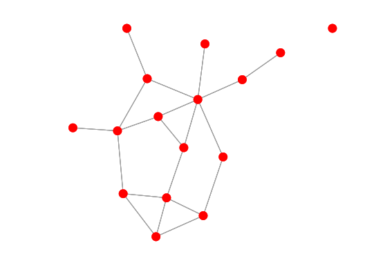
With no styling options, nwplot just shows the structure:

. nwwebuse florentine, nwclear

. nwplot flomarriage, scheme(s1network) export("plot_basic.svg") replace
Calculating node coordinates...
Plotting network...
Exporting graph to plot_basic.svg...
file plot_basic.svg saved as SVG format

Layouts

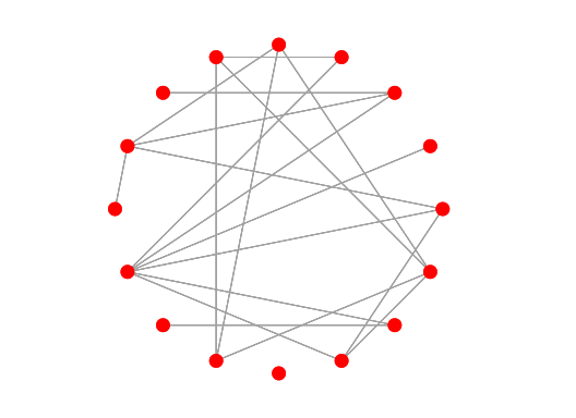
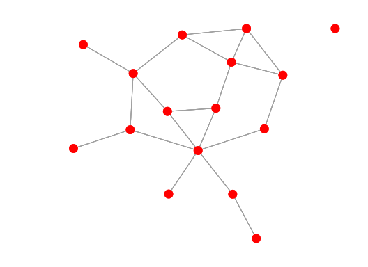
layout() controls how nodes are positioned. circle places every node on a ring; kk (Kamada-Kawai) is a force-directed layout that pulls connected nodes closer together:

. nwplot flomarriage, layout(circle) scheme(s1network) export("plot_circle.svg") replace
. nwplot flomarriage, layout(kk) scheme(s1network) export("plot_kk.svg") replace

layout(circle)	layout(kk)

On a valued network the layouts kk and frucht use the tie values as strengths (since nwcommands 3.10.0, as igraph::plot() does for a graph with a weight attribute): strongly tied nodes lie closer together, and the edge widths show the same values. The option binary draws the layout from the pattern of ties only, as earlier versions did. A network with negative values keeps the layout of the pattern, and so do the layouts circle, mds, hierarchy and bipartite.

Styling by attribute

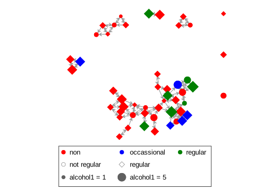
color(), symbol(), and size() each take a variable and map its values onto the plot:

. nwwebuse glasgow, nwclear

. nwplot glasgow1, color(smoke1) symbol(sport1) size(alcohol1) scheme(s1network) export("plot_styled.svg") replace
Calculating node coordinates...
Generating splines...
Plotting network...
Exporting graph to plot_styled.svg...
file plot_styled.svg saved as SVG format

Schemes

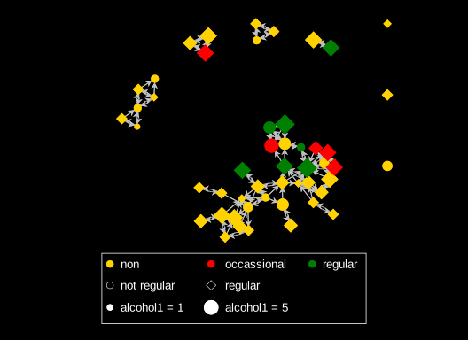
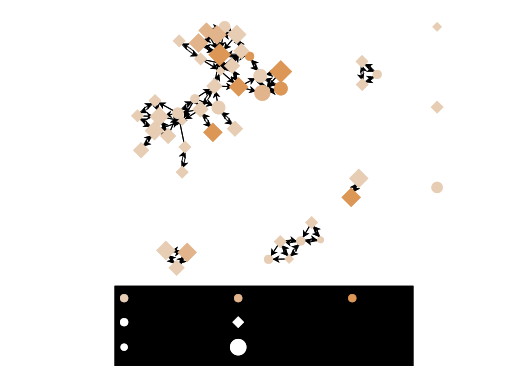
nwcommands ships three schemes purpose-built for network plots — s1network (used above), s2network, and s3network — each giving node fill and edge line colors that are visually distinct by default:

. nwplot glasgow1, color(smoke1) symbol(sport1) size(alcohol1) scheme(s2network) export("plot_scheme2.svg") replace
. nwplot glasgow1, color(smoke1) symbol(sport1) size(alcohol1) scheme(s3network) export("plot_scheme3.svg") replace

scheme(s2network)	scheme(s3network)

Highlighting a path

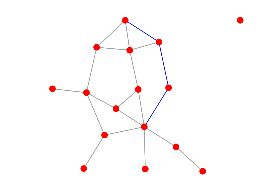
Combining nwpath with edgecolor() highlights a specific route through the network — here, the shortest path between two Medici-era Florentine families. nwpath’s generate() creates a new network per shortest path found (sp_1 here - a pair with multiple shortest paths would also get sp_2, sp_3, …), and that new network can be passed straight to edgecolor():

. nwwebuse florentine, nwclear

. nwpath flomarriage, ego(medici) alter(peruzzi) generate(sp)

----------------------------------------
  Network: flomarriage
----------------------------------------
    Ego                  : medici
    Alter                : peruzzi
    Shortest path length : 3
----------------------------------------
  Path 1: medici <=> barbadori <=> castellani <=> peruzzi
  Path 2: medici <=> ridolfi <=> strozzi <=> peruzzi

. nwplot flomarriage, edgecolor(sp_1, legendoff) scheme(s1network) export("plot_path.svg") replace

Don’t reach for edgesize() here to make the path stand out further - it scales edge width proportionally to the variable’s own value, so a 0/1 indicator like sp_1 makes every non-path edge exactly zero-width (invisible), leaving only the path on the plot. edgecolor() alone is the right tool for a discrete highlight/no-highlight distinction like this.

What the plot shows by default for valued, signed and two-mode networks

The networks above are binary, so every tie looks the same. Since version 3.9.0 nwplot shows more when the network is not binary, without any option:

• Valued network: the tie values set the widths of the lines (one to four units, the largest absolute value widest). binary draws all lines equally wide; edgesize() chooses the variable or the width range yourself.
• Signed network (a valued network with negative ties): positive ties are solid navy lines and negative ties dashed cranberry lines, with a legend; the width follows the absolute value. nosign switches the colours off, and an edgecolor() of your own replaces them.
• Two-mode network: the two modes get different symbols (circle, diamond) and colours, with a legend, unless color() or symbol() is given. layout(bipartite) puts the two modes in two rows or columns (tutorial 11).

nwplotmatrix has a legend of the value classes in the same way (legend(off) removes it) and, for a two-mode network, puts the nodes of one mode next to each other with a line between the modes.

Interactive plots

interactive writes the plot as a self-contained web page (the drawing library is inside the file; nothing is sent over the Internet, so you can mail the page to a colleague). In the page you drag nodes to reposition them, click a color or shape swatch in the legend to recolor every node sharing that value, and move two sliders for the size of the nodes and the width of the lines. The glasgow plot below is the same view embedded live, so try it:

. nwwebuse glasgow, nwclear

. nwplot glasgow1, color(smoke1) symbol(sport1) scheme(s1network) interactive noopen fname(interactive_plot)
Calculating node coordinates...
Generating splines...
Preparing interactive view...
Interactive view written to .../interactive_plot.html
Plotting network...

. display "`r(fname)'"
.../interactive_plot.html

Without noopen, Stata opens the page in a small viewer window; with noopen it only writes the file. fname() says where: the name you give (.html is added if missing; a relative name is relative to the working directory, and an existing file is replaced). Without fname() the page is written to Stata’s temporary folder under a time-stamped name. Either way the path is displayed and returned in r(fname), and r(interactive) holds the same path.

Drag any node below to reposition it. Click a legend swatch to change the color assigned to that whole group.

The workflow: explore in the browser, finish in Stata

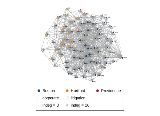
The browser is for looking at the network from several sides; the figure you publish is better made in Stata, where it can be reproduced. The steps, with the advice network of the 71 lawyers of the Lazega law firm (color for office, shape for practice, size for the number of colleagues who ask the lawyer for advice):

1. Build the page and keep the layout. generate(x y) stores the coordinates that nwplot computed; set seed makes the starting layout repeatable.
2. Work in the page. Drag, recolor, move the sliders, then use Save nodes and Save edges. They write two small CSV files (nwedit_nodes.csv, nwedit_edges.csv). The viewer window asks where to save them; in a browser tab they go to the Downloads folder.
3. Bring the edits back. nodexy(x y) tells nwplot where the nodes were, importcoords() and edgeimport() read the two files.
4. Export the static figure with export().

. nwwebuse lazega, nwclear

. quietly nwdegree lazega_adv, generate(outdeg indeg)

. set seed 42

. nwplot lazega_adv, color(office, colorpalette(navy dkorange gs12)) symbol(practice) size(indeg) label(_nwnode) edgefactor(0.4) generate(x y) interactive noopen fname(lazega_advice_interactive)
Calculating node coordinates...
Generating splines...
Preparing interactive view...
Interactive view written to .../lazega_advice_interactive.html
Plotting network...
Export coordinates...

The page this call writes is on its own page, Interactive demo: the Lazega advice network. Two CSV files saved in such a session (one node dragged, the Providence lawyers recolored, the size slider at 1.85) are in the folder of this tutorial; they bring the edits back like this:

. nwplot lazega_adv, nodexy(x y) importcoords("lazega_saved_nodes.csv") edgeimport("lazega_saved_edges.csv") color(office, colorpalette(navy dkorange gs12)) symbol(practice) size(indeg) label(_nwnode) scheme(s1mono) labelopt(mlabsize(tiny)) export("plot_lazega_bringback.svg") replace
(9 vars, 71 obs)
(4 vars, 892 obs)
Generating splines...
Plotting network...
Exporting graph to plot_lazega_bringback.svg...
file plot_lazega_bringback.svg saved as SVG format

Things to know about the bring-back:

• Sizes. The size slider in the page is a multiplier on the page’s own starting size, and the page draws in screen pixels. A slider value of 1 therefore corresponds to about nodefactor(0.2) in the static plot. Without nodefactor(), nwplot uses 0.2 times the saved slider value (1.85 gives nodefactor(0.37)), so the static figure has the proportions of the view. Give nodefactor() or edgefactor() yourself and your value wins over the saved one, for example to make the symbols smaller for a printed page.
• Same network. The edits are matched to the nodes and ties by row number, so run the bring-back on the same network, with the same sort order and the same if and in restrictions. A mismatch gives an error.
• Shapes. The shape drop-down in the legend belongs to a color group. When the nodes of a group have different shapes (here symbol(practice) is a second variable), it reads “mixed”. Choosing a shape there sets all nodes of the group. Read the legend drawn on the canvas for the shapes.
• Edge colors and patterns can be edited the same way and come back through edgeimport().

See nwplot for all options of the interactive view.

Movies

nwmovie turns a sequence of waves of the same network into a single, self-contained, browser-based timeline player — drag the slider and watch nodes and ties change wave to wave:

. nwmovie glasgow1 glasgow2 glasgow3, noopen fname(friendship_movie)
Resolving network glasgow1 (1/3)...
Resolving network glasgow2 (2/3)...
Resolving network glasgow3 (3/3)...
Wrote friendship_movie.html

Drag the timeline slider below to move between the three waves of the Glasgow friendship network.

Saving a movie as a video or GIF

The Export GIF and Export video buttons save the movie as it plays, with the wave readout drawn in. To write the file from a do-file instead, give export(); the extension sets the format (.mp4, .webm or .gif). A viewer window opens briefly, encodes the movie and closes again. Nothing else needs to be installed, on Windows, macOS or Linux.

. nwmovie glasgow1 glasgow2 glasgow3, duration(2000) export(friendship.mp4) replace
. nwmovie glasgow1 glasgow2 glasgow3, duration(2000) export(friendship.gif) replace

duration() is the time in milliseconds for each change from one wave to the next, so it sets the length of the video: two seconds per change give a four-second movie for three waves.