Tutorial 6: Generating Networks
Sometimes you don’t want real data at all — you want a network with known, controllable
properties, to teach a concept, test a method, or run a simulation against. nwcommands ships
four generators, each producing a different, well-studied kind of structure, and nwrandom can also
draw a random network in which every node has a degree you choose.
Random networks (Erdős–Rényi)
nwrandom gives every potential tie the same, independent probability of existing:
. nwclear

. nwrandom 15, prob(.2) undirected

. nwsummarize
--------------------------------------------------
   Network name:  random
   Network id:  1
   Directed: false
   Valued: false
   Two-mode: false
   Nodes: 15
   Selfloop: false
   Edges: 22
   Minimum value:  0
   Maximum value:  1
   Density:  .21
   Temporal: false
prob() leaves the exact tie count to chance — .21 density here, not exactly .2. Use
density() instead to fix the tie count exactly:
. nwrandom 15, density(.2) undirected name(randdens)

. nwsummarize randdens
--------------------------------------------------
   Network name:  randdens
   Network id:  2
   Directed: false
   Valued: false
   Two-mode: false
   Nodes: 15
   Selfloop: false
   Edges: 21
   Minimum value:  0
   Maximum value:  1
   Density:  .2
   Temporal: false
weights() assigns a value to each placed tie, independent of how the tie itself was placed —
here, weight 1 never occurs (probability 0.0), weight 2 occurs about 30% of the time, and
weight 3 about 70%:
. nwrandom 15, prob(.2) undirected weights(0.0, 0.3, 0.7) name(randval)

. nwsummarize randval
--------------------------------------------------
   Network name:  randval
   Network id:  3
   Directed: false
   Valued: true
   Two-mode: false
   Nodes: 15
   Selfloop: false
   Edges: 19
   Minimum value:  0
   Maximum value:  3
   Density:  .181
   Temporal: false
Small-world networks (Watts–Strogatz)
nwsmall starts from a ring lattice — every node tied to its k nearest neighbors on each
side — then rewires a fraction of those ties at random. The result keeps the ring’s local
clustering while a few long-range “shortcuts” dramatically shrink the distance between distant
nodes — the classic “small-world” effect:
. nwsmall 20, k(2) prob(.1) undirected

. nwsummarize
--------------------------------------------------
   Network name:  small
   Network id:  4
   Directed: false
   Valued: false
   Two-mode: false
   Nodes: 20
   Selfloop: false
   Edges: 40
   Minimum value:  0
   Maximum value:  1
   Density:  .211
   Temporal: false

. nwplot, layout(circle) scheme(s1network) export("plot_smallworld.svg") replace
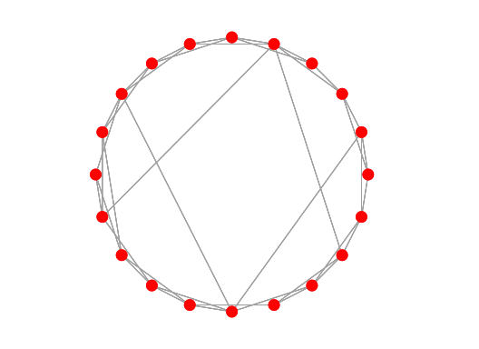
Laid out on a circle, most ties stay short (connecting near-neighbors on the ring), with a handful of longer chords cutting across — those are the rewired shortcuts.
Preferential attachment (Barabási–Albert)
nwpref grows a network one node at a time: each new node is more likely to connect to
already-well-connected nodes than to obscure ones. This “rich get richer” dynamic produces a
characteristic hub structure — a few nodes accumulate far more ties than the rest:
. nwpref 20, undirected

. nwsummarize
--------------------------------------------------
   Network name:  pref
   Network id:  5
   Directed: false
   Valued: false
   Two-mode: false
   Nodes: 20
   Selfloop: false
   Edges: 37
   Minimum value:  0
   Maximum value:  1
   Density:  .195
   Temporal: false

. nwdegree, generate(deg)
----------------------------------------
  Network name: pref
----------------------------------------
    Degree distribution

        deg |      Freq.     Percent        Cum.
------------+-----------------------------------
          2 |         11       55.00       55.00
          3 |          2       10.00       65.00
          5 |          3       15.00       80.00
          6 |          1        5.00       85.00
          7 |          2       10.00       95.00
         11 |          1        5.00      100.00
------------+-----------------------------------
      Total |         20      100.00

   Degree centralization: .427

. sort deg _nwnode

. list _nwnode deg in -5/-1

     +---------------+
     | _nwnode   deg |
     |---------------|
 16. |      n8     5 |
 17. |      n3     6 |
 18. |      n2     7 |
 19. |      n4     7 |
 20. |      n1    11 |
     +---------------+
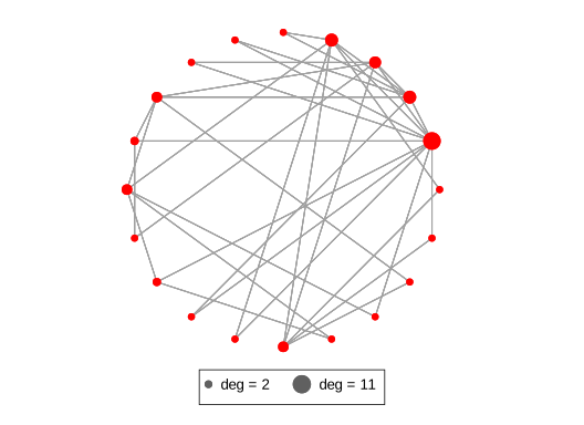
Over half the nodes have only degree 2, while n1 — one of the earliest nodes, and so one of the
first eligible targets for every later arrival — ends up with degree 11. Sizing nodes by degree
makes the hub visible directly:
. nwplot, layout(circle) scheme(s1network) size(deg) export("plot_prefattach.svg") replace
Lattice networks
nwlattice generates a plain structured grid — no randomness at all — useful as a baseline or
for teaching (e.g. contrasting a regular structure against the random/small-world/preferential
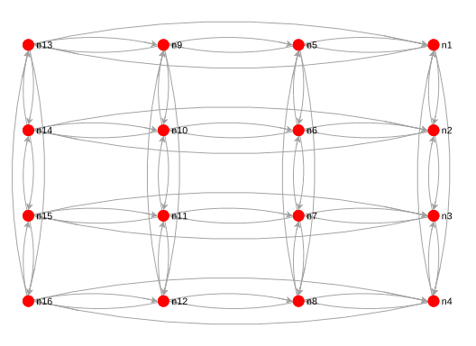
ones above). xwrap/ywrap wrap the grid’s edges around so every node has exactly 4 neighbors:
. nwlattice 4 4, xwrap ywrap

. nwsummarize
--------------------------------------------------
   Network name:  lattice
   Network id:  6
   Directed: true
   Valued: false
   Two-mode: false
   Nodes: 16
   Selfloop: false
   Arcs: 64
   Minimum value:  0
   Maximum value:  1
   Density:  .267
   Temporal: false

. nwplot, layout(grid) label(_nwnode) scheme(s1network) export("plot_lattice.svg") replace
Random networks with given degrees
Real networks rarely have the degrees of an Erdős–Rényi network: a few nodes have many ties and many have
few. nwrandom with degree() draws a network in which every node has exactly the degree you give
and the ties are otherwise random (no loops, no pair tied twice). It first builds one network with these
degrees and then exchanges the partners of two ties at random many times (the
sample_degseq(method = "edge.switching.simple") of igraph). degree() takes a list of numbers or a
variable:
. set seed 2026

. nwrandom 8, degree(3 3 2 2 2 2 1 1) name(randdeg)

. nwdegree randdeg, generate(d_randdeg)
----------------------------------------
  Network name: randdeg
----------------------------------------
    Degree distribution

  d_randdeg |      Freq.     Percent        Cum.
------------+-----------------------------------
          1 |          2       25.00       25.00
          2 |          4       50.00       75.00
          3 |          2       25.00      100.00
------------+-----------------------------------
      Total |          8      100.00

   Degree centralization: .19

. list _nwnode d_randdeg in 1/8, noobs

  +--------------------+
  | _nwnode   d_rand~g |
  |--------------------|
  |      n1          3 |
  |      n2          3 |
  |      n3          2 |
  |      n4          2 |
  |      n5          2 |
  |--------------------|
  |      n6          2 |
  |      n7          1 |
  |      n8          1 |
  +--------------------+
Not every list of degrees can be the degrees of a network. Three nodes with one tie each would need one
and a half ties, and nwrandom says so:
. capture noisily nwrandom 3, degree(1 1 1) name(bad)
No network without loops and repeated ties has these degrees (their sum must be even, and
> no degree can exceed 2; see the Erdos-Gallai conditions).
invalid syntax
The most useful degrees are those of a real network. Random networks with the degrees of the Florentine marriage network show what the degrees alone produce. The global clustering coefficient of the families is .19; the random network with their degrees has .13:
. nwwebuse florentine, nwclear

. nwdegree flomarriage, generate(d_flo)

. nwrandom 16, degree(d_flo) name(floran) xvars

. nwclustering flomarriage, generate(cc1) replace
----------------------------------------
  Network name: flomarriage
----------------------------------------
    Measure: binary
    Average clustering coefficient: .218
    Global clustering coefficient: .191

. nwclustering floran, generate(cc2) replace
----------------------------------------
  Network name: floran
----------------------------------------
    Measure: binary
    Average clustering coefficient: .118
    Global clustering coefficient: .128
One random network proves little. Many of them, compared with the observed value, make a test:
nwcug with condition(degrees) does exactly that (Tutorial 18). For a directed
network give outdegree() and indegree() (for example the variables of nwdegree); every node then
keeps both. To rewire an observed network instead of starting from a list, use nwpermute with swap
(nwpermute), which also carries tie values along.