Tutorial 1: A latent space for the karate club
Goal. Fit a latent space model with nwlsm, read the posterior summaries, check that the sampler has converged, and judge whether the model reproduces the network.
Data. Zachary’s karate club: 34 members of a university karate club and 78 friendship ties (undirected). Source: Zachary, W. W. (1977), Journal of Anthropological Research 33, 452-473;
loaded from the website with nwwebuse zachary (see the data sets page). You need the core nwcommands and the nwlsm package (see Install); the commands were run with nwlsm 1.0.0 under Stata 17.
The complete script and log are in example.do and example.log.
What a latent space model does, in five sentences
Every actor has an unobserved position in a space with a few dimensions (here two, a plane). The probability of a tie between two actors falls as the distance between them grows: the log odds of a tie are an intercept minus the distance. Given the positions, the ties are independent, which is all the model assumes. Because distance obeys the triangle inequality, friends of friends are close to each other, so the model produces clustering without being told to. The positions are not observed and are estimated together with the intercept, by Markov chain Monte Carlo, which delivers a sample from the posterior distribution (the draws) instead of one number per parameter.
Fit
. nwwebuse zachary, nwclear
. nwlsm zachary_bin, dim(2) nsample(2000) burnin(5000) interval(10) chains(2) seed(20261120)
------------------------------------------------------------------------------
Latent space model (Euclidean distance; bernoulli family), posterior by MCMC
Network: zachary_bin (34 actors, undirected)       Latent dimensions: 2
Draws: 2000  burn-in: 5000  interval: 10           Seed: 20261120
Chains: 2 (1000 draws each, pooled)
Posterior mean log likelihood:  -170.621 (sd  7.596)
------------------------------------------------------------------------------
                              Mean        Sd   MC s.e.  Lower 95% Upper 95%
------------------------------------------------------------------------------
_cons                       1.0127    0.3748    0.0271     0.3151    1.7703
------------------------------------------------------------------------------
Variance parameters (posterior):
sigma2                      4.6310    1.5218    0.0955     2.2146    8.3254
------------------------------------------------------------------------------
Acceptance rate of the latent positions: 0.239
Gelman-Rubin statistic: largest value  1.005 (see estat mcmcdiag)
Positions: minimum Kullback-Leibler estimate e(Z) (also estat positions); mean
of the draws aligned to it e(Zmean); posterior mean distances e(D); posterior
mean tie probabilities e(P). Positions are identified up to rotation,
reflection and translation only.
nsample(2000) keeps 2,000 draws, chains(2) runs two independent chains of 1,000 each, and seed() makes the fit reproducible (for a given seed the result is the same for any number of threads).
The table reports, for every parameter, the posterior mean and standard deviation, the Monte Carlo standard error (the error of the mean due to the finite number of draws) and a 95% credible interval.
The intercept is 1.01: with no distance between two actors, the log odds of a tie would be about 1. The variance of the positions (sigma2) says how spread out the actors are in the latent space.
The acceptance rate of the positions (0.24) is near the value that makes a random-walk sampler efficient; nwlsm tunes the step sizes to reach it.
Did the sampler converge?
. estat mcmcdiag

MCMC diagnostics (2000 draws in 2 chains, interval 10)
--------------------------------------------------------------------------
Parameter                Mean       Sd      ESS ESS/draw Geweke z     Rhat
--------------------------------------------------------------------------
_cons                  1.0127   0.3748    160.8    0.080    -0.73    1.005
loglik              -170.6210   7.5961    263.2    0.132    -1.47    1.001
sigma2                 4.6310   1.5218    229.0    0.114    -0.72    1.003
--------------------------------------------------------------------------
Acceptance rates: positions 0.239, _cons 0.233
ESS: effective sample size by the initial monotone positive sequence
estimator.
With 2 chains: ESS is the sum over the chains, Geweke z (above) the value of
largest size over the chains, Rhat the Gelman-Rubin potential scale reduction
factor (values close to 1, say below 1.1, indicate that the chains agree).

Geweke z by chain
------------------------------
Parameter       chain1  chain2
------------------------------
_cons            -0.73   -0.69
loglik           -1.47   -1.46
sigma2           -0.72   -0.58
------------------------------
Geweke z: first 10% of the draws against the last 50%, as geweke.diag() of R's
coda (spectral density at frequency zero of each part from an autoregressive
fit); |z| > 1.96 is the nominal two-sided 5% limit. 0 of the 6 z values (3
parameters, 2 chains) exceed it (largest |z| 1.47); about 0.3 (5%) would
exceed it by chance with long settled chains, and more with short chains (a
first part of a few dozen draws gives a noisy z), so read the z values
together with the trace plots (graph) and the effective sample sizes; they are
no test of convergence.
Look at the last column. The Gelman-Rubin statistic compares the chains with each other; values near 1 (below 1.1) mean that they agree. The effective sample size (ESS) says how many independent draws the 2,000
correlated draws are worth, here between 160 and 260, which is enough for the means but small for the tails of the intervals; a longer run (nsample(), interval()) raises it. The Geweke z compares the mean of the first 10% of a chain with that of the last 50% (the value is the one of R’s coda::geweke.diag()), and the second table gives it for every chain. It is informational and no test of convergence: with several short chains a few z values beyond 1.96 are normal, and the footnote counts them. Here none of the 6 does. With real data, run at least two chains and look at these numbers together with the trace plots (estat mcmcdiag, graph) before looking at anything else.
The positions
. estat positions

Positions of the actors (minimum Kullback-Leibler estimate)
--------------------------------------
Actor               dim1        dim2
--------------------------------------
r1               -0.8032     -0.1903
r2               -0.7085     -0.2280
r3               -0.2556     -0.1406
r4               -0.7419     -0.2159
r5               -1.8200      0.5175
r6               -1.8975      0.7206
r7               -1.8975      0.7206
r8               -0.7419     -0.2159
r9                0.3700     -0.1619
...
The reported positions are the minimum Kullback-Leibler positions of latentnet: the positions whose tie probabilities are closest to the posterior mean tie probabilities. They are identified only up to rotation, reflection and
translation, so only the distances between actors mean anything, never the axes. nwlsmplot draws the network in the latent space, and the option clusters(#) with estat clusters finds groups of actors that lie together.
A table of coordinates is hard to read. nwlsmplot draws the same positions as a map, with the ties of the network as light lines:
. nwlsmplot, title("The karate club in the latent space")
. graph export "karate_positions.png", width(900) replace
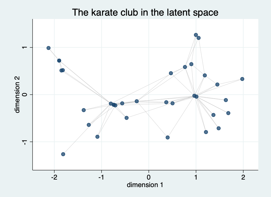
Actors that are tied sit close together, and actors without ties in common lie far apart. Two actors, one in the middle left and one in the middle right, hold most of the ties, and the others lie around them. A few actors have exactly the same position in the table above because they have the same ties; they are drawn on top of each other. Read the map by distances only: turning or flipping it would change the axes and nothing else. Both axes have the same scale (one unit is equally long horizontally and vertically), so distances can be read directly from the picture; noequal switches this off and lets each axis span its own range. The option clusters colours the actors by latent cluster once the model has been fitted with clusters() (tutorial 2).
The map shows one point per actor, but each position is an estimate. The option draws(#) adds the uncertainty: it draws that many of the kept posterior draws of all positions, aligned to the minimum Kullback-Leibler positions, as small faint dots in the colour of the actors under the map:
. nwlsmplot, draws(100) title("The karate club with 100 posterior draws of the positions")
. graph export "karate_draws.png", width(900) replace
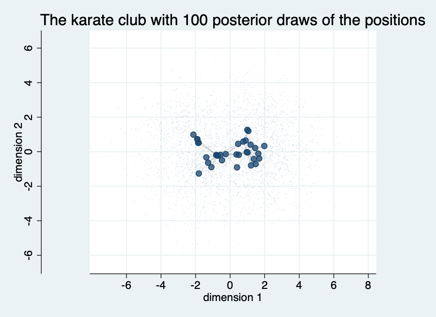
The estimated positions (the dark points, with the ties as thin lines) now sit in a small region in the middle of a much wider, faint cloud that reaches about 5 units from the centre in every direction (both axes have the same scale, so the cloud is drawn undistorted). The cloud is the union of 100 draws for each of the 34 actors, so it shows how far a single actor could lie in the posterior. It is wide compared with the distances between the estimated positions: the map of the minimum Kullback-Leibler positions is a tidy summary, but the data do not pin down the position of an individual actor, and the finer arrangement within the groups should not be over-read. The draws stay in memory until the next fit; if you fit another model first, draws() stops with an error.
Goodness of fit
. estat gof

Goodness of fit: degree (100 networks simulated from the posterior)
------------------------------------------------------------------
      Degree |  Observed       Min      Mean       Max  MC p-value
-------------+----------------------------------------------------
           0 |         0         0      0.98         4        0.70
           1 |         1         0      2.12         7        0.70
           2 |        11         1      3.91        10        0.00
           3 |         6         1      4.94        11        0.80
           4 |         6         1      5.46        12        0.94
           5 |         3         1      5.03        12        0.44
           6 |         2         1      4.25        10        0.22
           7 |         0         0      3.23         8        0.10
           8 |         0         0      1.98         8        0.26
           9 |         1         0      1.19         5        1.00
          10 |         1         0      0.48         2        0.76
          11 |         0         0      0.30         3        1.00
          12 |         1         0      0.10         2        0.18
          13 |         0         0      0.03         1        1.00
          16 |         1         0      0.00         0        0.00
          17 |         1         0      0.00         0        0.00
------------------------------------------------------------------
estat gof simulates 100 networks from the posterior and compares their degree distribution with the observed one (and, in further tables, the geodesic distances and other statistics).
The MC p-value is small for degree 2 (the club has 11 members with exactly two friends, a simulated network 3.9 on average) and for the two members with 16 and 17 friends, whom no simulated network reproduces.
A model with the random sociality effect, which gives every actor a propensity to have ties, is the natural next step for such hubs.
What to remember
- The Euclidean model describes the network by distances. It suits networks with clusters and transitivity, and fits poorly where a few hubs drive the degrees.
- Check the chains first (
estat mcmcdiag), then the fit (estat gof), then read the results. - Positions are a picture, not a measurement. Do not interpret the axes.
- For other approaches to the same kind of question see Which package do I need?; a stochastic block model of the same network is in the nwsbm tutorial.